Gen IV AI Training Guide

Overview

The purpose of this document is to provide general instructions and best practices for training new Gen IV AI models for defect inspection within nSpec scans. Particular focus will be spent on best practices for training models when defects examples are diffuse and spread out across many different wafers and scans. This adds some complexity to the AI training process, which by default is easiest when starting with a single folder full of example defects. Not every defect occurs in such high densities on a single wafer scan.

AI Model Training Steps

Training a new AI model can be broken down into three basic steps:

1. Capture New Scan Data

2. Extract New Training Examples

3. Label & Incorporate New Data into the Model

A fourth step is recommended for safe and reversible improvement of the model over time – after each new batch of defects is added in to the model, it is beneficial to save all progress by creating a new project version. This step can be performed at any point in time, but often makes the most intuitive sense between steps 2 & 3.

Once a new version of the model has completed training, the cycle can be repeated as many times as it takes to produce good results.

When to Train a New Model

When considering when to train a new AI model, consider the following: Do the images look different than the images that went into the trained model? If so, it is best practice to train a new AI model.

The following scenarios could require the training of a new AI model:

• Different Processing Layer

• Different Magnification

• Different Imaging Mode (BF, DF, DIC)

• Different brightness or exposure when scanning

It is possible that the Nanotronics AI could perform well across any or all of the above scenarios, however there is no guarantee – and this is important to consider when developing new inspection procedures within nSpec. AI is a new technology, and while we are rapidly developing its capabilities, it is still fallible. For best results, create a standard for how all images in your training set and images to be classified will look prior to embarking on the training process for maximum accuracy.

Modifications to how images look may potentially confuse the AI, so any changes to the above might cause a lower rate of defect detection, a higher rate of false positive detections, or a higher rate of misclassifications. Consider a 4 pixel particle defect scanned at 2.5x magnification. When the AI is trained to pick up that defect within a 2.5x brightfield image, it is 4 pixels. Now let’s say you scan that same defect at 50x – now it is about 100 times larger, 400 pixels across. That same defect looks very different when imaged differently, and it makes sense that that object doesn’t get identified as the same object from the perspective of the AI. Now let’s say you switch to darkfield imaging mode. Now instead of being a tiny dark object on a gray background, it’s a giant white object on a black background.

That said, it is possible that you could have luck starting from an existing trained model, and working from there. However, results can’t be guaranteed in that circumstance. Please let the Nanotronics team know if you have luck training our AI to work well across any of the dimensions listed above, we’d love to learn new techniques for make the most of our AI models.

Step 1: Capture New Data

Before doing anything, you’ll need to capture some initial data to use to train the AI. This should be as straightforward as capturing a single scan of your sample within nSpec. AI Inspection is relatively resilient to some of the pitfalls that can undermine other analysis methods: oversaturation of pixel intensity, small rotations of the sample, insufficient contrast, vignette of the image intensity across the field of view, etc. These can all commonly cause problems with other analysis methods. AI seems to handle these factors very well. Still, the better the quality of data that goes in to the AI analysis, the better the inspection will perform.

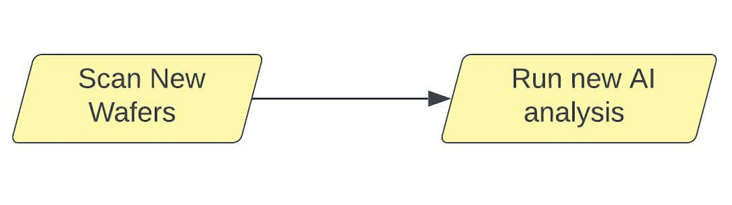
If this is the first iteration of training the AI, you may not have much analysis data to work from to find new example defects. Generally, it could help to start with one of the other Nanotronics analyzers just to find where defects exist on the wafer, unless defects are very abundant and easy to find. Device Inspection or one of the Basic Selection analyzers can really speed things up if defects are rare across the wafer. If this is not the first AI iteration, run the latest version of the AI analysis, and that will usually get you close to finding most defects across the wafer.

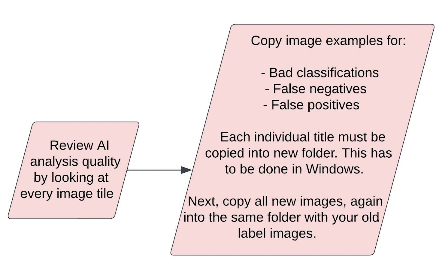
Step 2: Extract New Training Examples

Now that you have scan data, we need to find good examples of defects we’d like the AI to classify from these images. To do this, review the image set in nView, and copy all images of interesting defects into a new folder within Windows. With each new iteration, we recommend that you save the new training examples in a new folder for that specific iteration, while also maintaining a master folder of all defect training examples across all iterations.

Here’s our recommended workflow for extracting new training examples:

1. Open the scan inside nView.

2. Open the folder containing all the scan images in Windows Explorer.

3. In a new window, create a folder that will hold all defect examples from this iteration.

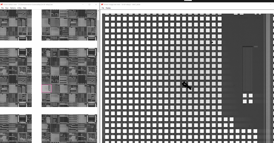
4. Look through the scan in nView. Once you find a good defect example:

   1. Find that image tile in the Windows Explorer.

   2. Copy (not cut) the image.

   3. Paste the image into your defect examples folder.

5. Continue looking through the scan in nView.

6. Repeat step 4 until you have at least:

   1. 10 different images for each defect class you intend to train the AI to recognize.

   2. 30 examples of each defect type (they can be in as few as 10 images, or spread across more images if each tile only contains a single example of that defect.

   3. 50 images total.

7. If this is your first iteration of model training, create a master folder to contain all defect image examples used to train the AI model across all iterations.

8. Copy all of the new defect images from the current iteration into your master folder of all defect image examples.

   1. Keeping the separate folder is optional, but recommended for troubleshooting.

You may be able to start with fewer example images, however this is the recommendation for a performant AI model.

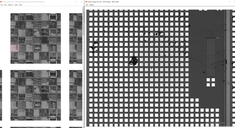
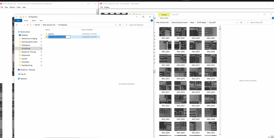
Here is a visual walkthrough of what this might look like on your wafer.

1. Open new scan in nView.

2. Open folder containing scan images in Windows Explorer.

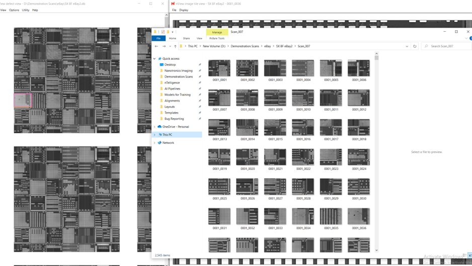
3. Create folder to hold defect examples from the current iteration in a new window.

4. Find interesting defect, then copy it to your example folder in Windows.

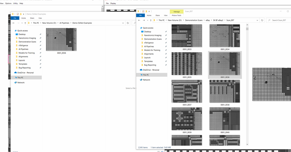
5. Continue searching for defect examples in nView.

6. Continue until you have at least 50 images.

Step 3: Configure New nTelligence Project Iteration

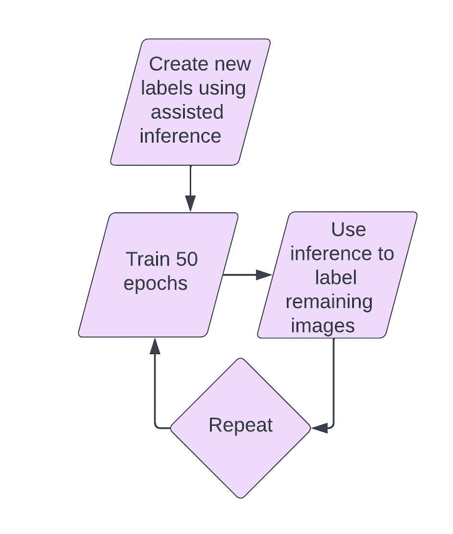
Anytime you add a new batch of defect examples to an AI model, it is recommended that you create a new project so that your work is reversible. This is most helpful at the beginning, as you learn what works best for your specific samples when training the Nanotronics AI. Here’s what this looks like when iterating on an existing AI model:

If you are starting on the first iteration of a new model, the first step above isn’t necessary since you don’t have any labels yet. If you are working off a previous example, before starting the new project, first you should export labels from the most recent iteration of your project.

Steps for project configuration:

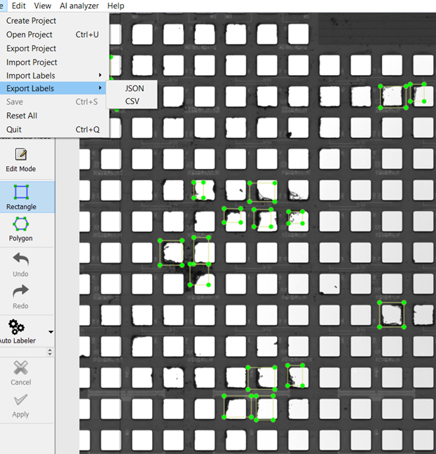
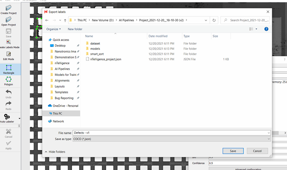
1. [Skip if training first iteration of new model] In the latest AI project, export your labels as JSON.

   1. Name them according to the current AI model version (v1).

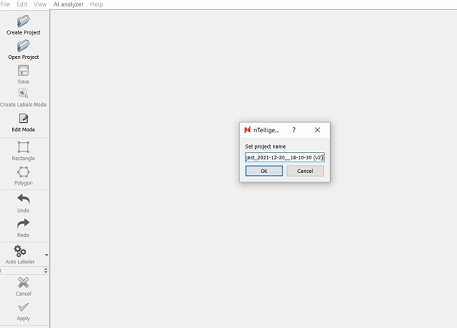
2. Create a new project in the same directory as your last project.

   1. Keep the timestamp version, but add a (v2) or appropriate version number to the end. This is very helpful for keeping track of your model training progress.

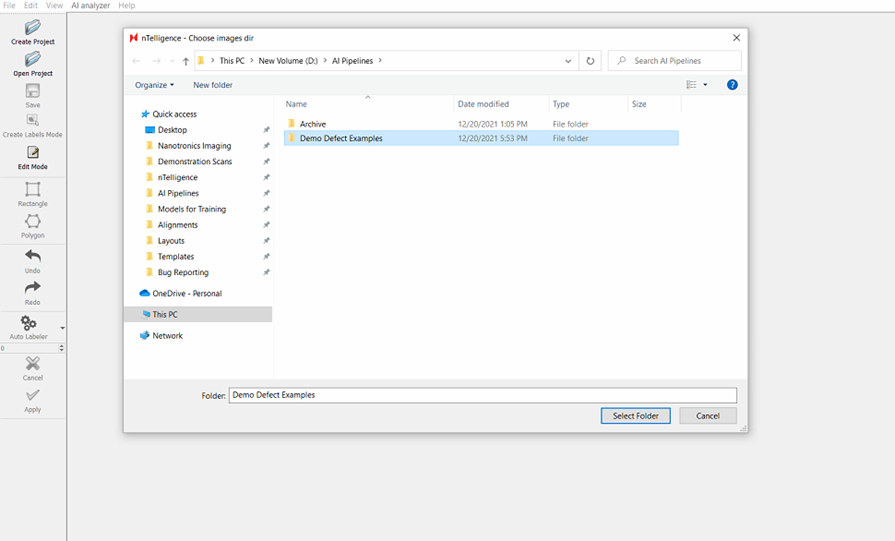
3. Point the project at the folder containing all your defect example images, not the folder that only contains the new example images.

4. When configuring the model, point at the output from your previous round of AI training.

5. Add your previously trained model to the auto-labeler.

Now you can move on to the next step.

Before we move on, here’s a visual walkthrough of what these steps look like:

 1. Open previous project, export your labels.

2. Name project into the same working directory as your last project, with the timestamp naming convention and a version number.

3. Point at your merged defect example folder as your images directory.

Step 4: When setting up the training model, point at resnet50 model from previous iteration. If it’s the first iteration of training, use the resnet50 model provided by Nanotronics.

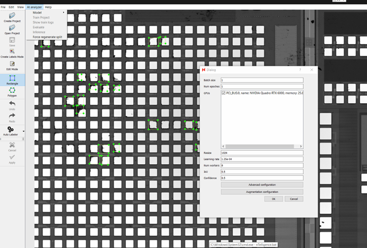
After choosing the model, a dialog will appear with AI training parameters.

Step 5: Add the previous model to the auto-labeler.

Step 4: Label New Images

Now that we have performed the following steps:

1. Scanning new data.

2. Sifting through those images for new defect examples & adding them to our training images.

3. Preparing a new project.

It is finally time to label the new examples. There are a few rules of thumb you should consider when labeling new classes of defects.

Choose classes describing defects that look visually similar

In general, try to separate your classes by defects that generally look similar to each other. This seems like common sense, but is an important point to make, because this might differ from how your inspection team typically categorizes defect classes. Keeping this in mind can improve the speed at which a new model can be trained, as well as its ultimate accuracy to identify & classify defects within the unique context of your scans.

Here’s an example:

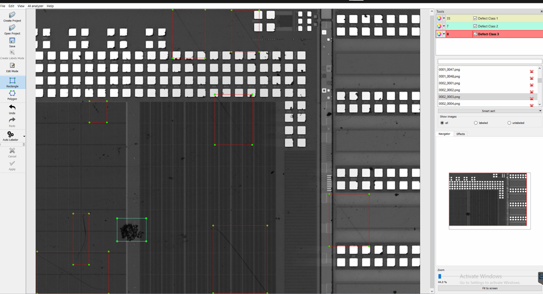
In this example, scratches (Defect Class 3) and Large Particles (Defect Class 2) are very visually distinct. One is long and skinny, and the other is a big dark blob. However your process might categorize both of these defects as “Surface Defect.” If you created a single “Surface Defect” class that contained both of these examples, the model might take a long time to train, with many hundreds of image examples, before it performs well. This is because those defects look as different to the AI as they do to us.

For this reason, it is recommended that you classify based on visual presentation of defects, rather than a strict class naming convention based on a one-to-one mapping of your process categorizations. Usually, the two are one and the same, since as humans we tend to name things based on how they look. However this isn’t always the case, so it is important to mention. With enough examples, the AI will eventually learn that both of the above fall under a single class, but it could take a long time and many hundreds of examples to train a model that bins this way.

If you label one defect on an image, you must label them all

Another important note when labeling images, and this cannot be stressed enough, if you label a single defect on an image tile, you must label every single defect present on that image tile. There are algorithmic reasons for this, and we wish it weren’t the case because it complicates the training process. By not labeling a defect, you are effectively labeling that object as “not a defect.” This can undermine your previous hard work training that type of defect, and can cause the next iteration of the AI model to miss these defects. 

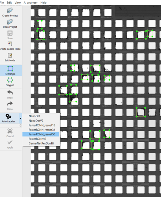
Use the auto-labeler to quickly add new labels

If you have a previous model loaded into the auto-labeler, you can click the auto-labeler button and the model will automatically find everything in the image and add labels. Your model is a work in progress however, so you will usually need to edit a few of its outputs. This is also a convenient way to gauge how well the model is performing so far. Initially, all the labels will be purple. Once you accept them, they will display the color that corresponds to each of your classes.

Once you have labeled all of your newly added defects, it is time to incorporate those new defects into your model by training again. Check that you have loaded your previous resnet50 model from your last version (or the starter model). It is recommended to train 50 to 100 epochs when incorporating a new batch of examples. Then, click Train Project.

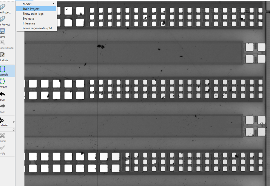
The training process can take some time, and duration is largely a function of the available GPU power on your system. If training takes more than 1 day, contact Nanotronics support. On most standard new Nanotronics systems, 50-100 epochs should take 1-3 hours to completely train. When it completes, a window should appear notifying you that training is complete. The command prompt will also state that training is complete, and that it reached the number of epochs specified when setting up the model within nTelligence.

Step 5: Repeat Until the AI Performance is Satisfactory