
nSpec v0.23.0.0 External Release Notes
nSpec Version 0.23.0.0
Release Date:
Documentation Updated:
Major Features: Support for nSpec Turbo and nSpec PRISM, Defect Classification Workflow, Improved Surface Prediction
Overview
nSpec v0.23.0.0 is one of Nanotronics’s biggest software releases. This release contains software support for two new nSpec products, nSpec Turbo and nSpec PRISM. nSpec Turbo features substantial performance upgrades to the hardware, increasing scanning speed, while nSpec PRISM has new ultraviolet and infrared illumination modalities, and allows for vast options and new workflows involving novel excitation sources. Additionally, this release includes support for new nSpec upgrades: any nSpec can be wrapped in a CleanCube, a clean environment enclosure including interlocks and ionizers, and nSpec now supports multiple load ports for different sample form factors within a single tool. Please reach out to our sales team regarding our latest automated handling capabilities at sales@nanotronics.co.
On top of these new products and capabilities, this release contains loads of new features and analyzers to improve existing workflows, including a powerful defect classifier tool that enables defect classification with trained AI models, improved user interfaces for the imaging settings dialog, and an overhaul of surface prediction algorithms.
Upgrading to v0.23.0.0
Library Updates Required
If upgrading from a version more than 1 release prior, please reference all intermediate release notes for upgrade steps for each version.
Compatibility Updates
nTelligence Gen II and Gen III AI Deprecation
Starting with nTelligence v5.0.0.4, which is bundled with nSpec v0.23.0.0, Gen II and III AI will be deprecated and replaced by Gen IV AI. Please contact Nanotronics support@nanotronics.co for assistance with upgrading any jobs that utilize Gen II or III AI.
Nikon Illuminator Deprecation
As of nSpec v0.23.0.0 support for Nikon systems is deprecated and no longer supported. The latest supported version for Nikon systems is v0.22.1.5. Please contact sales@nanotronics.co for options for getting onto v0.23.0.0.
Surface Prediction Algorithm Deprecation
In nSpec v0.23.0.0, the number of surface prediction algorithms has been greatly reduced and simplified. A number of less performant algorithms have been deprecated and point to new algorithms. The deprecated algorithms include PreFoc LI, PreFoc RT, PreFoc LP, PreFoc SP, PreFoc CW, PreFoc Triangular Advanced, PreFoc 3PP.
The table below shows the old deprecated algorithms and the new algorithms they have been mapped to. These mappings are automatically applied in v0.23.0.0.
Deprecated Algorithm | New Algorithm |
|---|---|
PreFoc LI | PreFoc Polynomial Standard |
PreFoc RT | PreFoc Triangular Standard |
PreFoc LP | PreFoc Triangular Standard |
PreFoc SP | PreFoc Triangular Standard |
PreFoc CW | PreFoc Triangular Standard |
PreFoc Triangular Advanced | PreFoc Triangular Standard |
PreFoc 3PP | PreFoc Triangular Standard |
Breaking Changes
NSPEC-5189: Wafer-skipping behavior when running job locally
Prior to nSpec v0.23.0.0, the use of a semicolon in the Sample name or Sample ID fields indicated wafer-skipping behavior. Starting with nSpec v0.23.0.0, only _SKIP_ will indicate wafer-skipping behavior, and using a semicolon will no longer indicate skipping.
NSPEC-7493: Scan Error Behavior
The old logic of the program option Sample Error Also Fails Cassette is modified in v0.23.0.0. The old behavior allows a cassette scan to finish to processing a sample when:
Sample Error Also Fails Cassette=1Job Error Also Fails Sample=0
Now, when Sample Error Also Fails Cassette = 1, a job error should always fail a sample, regardless of what Job Error Also Fails Sample is.
Hardware Updates
Trigger Interface Board
A new trigger interface board will be added to all machines during upgrading for increased camera stability.
Major Enhancements
nSpec v0.23.0.0 contains loads of major product enhancements, including:
nTelligence v5.0.0.4
Reclassifier Tool
Defect Classifer
Surface Prediction Algorithms
Kriging Surface Predictor
Flat Plane Surface Predictor
Imaging Settings Dialog Updates
Device Layout Editor Updates
Sample Naming and Wafer Skipping Behavior
nTelligence v5.0.0.4
Overview
There are many exciting new updates in the nTelligence v5.0.0.4 software release, including the addition of new models, the deprecation of Gen III AI, and a new and improved labelling workflow. Note that nTelligence 5.0.0.4 has a minimum GPU requirement of 10 GB.
Add Images to Project after Creation
Users can now add image directories to their nTelligence projects after project creation. Previously, users could only choose one image directory to work from during project creation. After opening or creating a project, users can import more images via File > Import Images > Image Directory. Note that once a folder is added, it cannot be deleted.
Gen III AI Deprecation
Starting with nTelligence v5.0.0.4, Gen III AI models are deprecated. All Gen III AI models must be converted to Gen IV AI models to be used with nTelligence v5.0.0.4. To convert your models, please contact Technical Services at support@nanotronics.ai.
Gen IV AI Model Files
nTelligence 5.0.0.4 includes new AI models that can be used to train AIs for classification of defects, on top of existing defect detection models.
Base Model Files
When receiving an nSpec tool, there should be a folder at D Drive > AI Pipelines > Base Models that contains base AI training models in .nano format to train new detection models on. We highly recommend making a copy of these models before your first time using nTelligence. It is easy to accidentally overwrite these, but if you do, Nanotronics support can always send you the original model files.
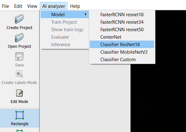
Note that when accessing the base models via AI Analyzer > Models, these options do not actually point at specific models, they are simply referencing the base model files. To actually utilize the listed base models in the menu options, you can click on any of the menu options, which will open a file dialog. The file chosen during this step is the actual model you are referencing, not necessarily the menu option chosen.
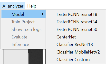
Screenshot of AI Analyzer → Model menu options in nTelligence v5.0.0.2
The first four models, FasterRCNN - ResNet50, FasterRCNN - ResNet34, FasterRCNN - ResNet18, CenterNet, are all detection models, meaning they are best suited to identifying where defects occur in an image. Note that these do have base .nano files, but the classification models do not have associated base model .nano files.
The remaining classifier models, Classifier ResNet18, Classifier MobileNetV2, Classifier Custom,are best suited to distinguishing defect classes from one another. These models should be trained on images of cropped defects, which can be obtained through Device Inspection Analysis. Again, these classification models are trained from scratch and do not have associated base model files.
Detection Models
Our recommendation is to begin training on the FasterRCNN - ResNet50 model. However, if you don’t have enough data, or if the data is too simple, it is possible that the model will be overfit.
“Simple” data means that the classes you are training to detect are easy to distinguish, for example, it is very easy to distinguish a defect that looks like a tiny dot from one that looks like a giant blob. The harder it is to distinguish defect classes, the more parameters the model should have. ResNet50 has the most parameters, followed by ResNet34 and ResNet18.
If you have simpler data or less training data, we recommend trying the lower numbered ResNet models, like FasterRCNN - ResNet34 and FasterRCNN - ResNet18, which have fewer parameters. They are smaller models with less layers, meaning they will train faster and be less prone to overfitting if your data set is smaller and simpler. CenterNet also trains faster than FasterRCNN - ResNet50.
Note on Overfitting
Overfitting occurs when an AI model does not have enough or representative training data, and as a result, the model performs extremely well on training data and very poorly on new data. This occurs because the model parameters memorize or mimic the training data.
Classification Models
Our recommendation for a classification model is Classifier ResNet18. You can try Classifier MobileNetV2 and Classifier Custom as well – preliminary internal testing has shown that ResNet18 gives best results.
The classification models are used to distinguish defects from one another, with the inputs being images of cropped defects, as opposed to full scan images used as training data for defect detection.
Reclassifier Tool
Partner-only. This document should not be shared with customers.
Overview
Starting with nTelligence v5.0.0.4, users can train AI models to classify defects, in addition to nTelligence’s existing ability to train AI models for defect detection. This is a huge step forward, and will make defect classification much more fast and efficient. At the core of this new workflow is the Defect Classifier Analysis, which as input takes the analysis results from a computer vision-based analysis like Basic Selection or Device Inspection, which detect all scanned anomalies, and a Defect Classifier nJson file, which points to a model trained to classify specific defects of interest.
Training an AI Classification Model in nTelligence
To use the Defect Classifier Analyzer, a classification model must be trained with labelled training data. This training data can be obtained by performing a scan with a computer vision based analysis like Basic Selection or Device Inspection in nSpec. After the scan is performed, the training data needs to be labelled in nTelligence, either manually or with the new Reclassifier Tool described below.
Note that the workflow below for labelling data including nReview is a temporary workflow, and will be replaced in an upcoming patch release with a much more easy to use workflow.
The Reclassifier Tool is an exciting new feature of nTelligence v5.0.0.4 that will help save loads of time labelling and classifying defects. The tool makes manual labelling much faster than before.
Labelling Data
There are a few steps that need to happen in order for the scan and analysis results to be properly handled by the Reclassifer Tool within nTelligence. This requires the use of a utility called nReview, which is not included in nSpec installation. Please contact support@nanotronics.co to get access to this utility.
nReview does a scan of all of the nSpec analysis results on the nSpec machine and visualizes them in an easy to access way. For each analysis result, there are two buttons, Open and Label.
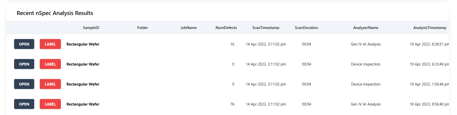
Folder and JobNames have been redacted for privacy reasons.
Clicking Open will open up nView. Clicking Label will generate a labels.db file in C: Nanotronics Imaging > nReview. This database file generates a categories table that shows all of the defects in this analysis labelled as Defect. Note that every time you press the Label button, the results for the analysis pressed will be appended to the existing labels.db file. This means that the results of multiple analyses can be combined into a single labels.db file.
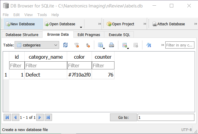
Now, this labels.db file needs to be moved into the nTelligence project folder created for this analysis. The file path from your nTelligence project folder should be [Insert your nTelligence project folder name] > dataset > labels. The existing labels.db file should be replaced by the one generated by nReview.
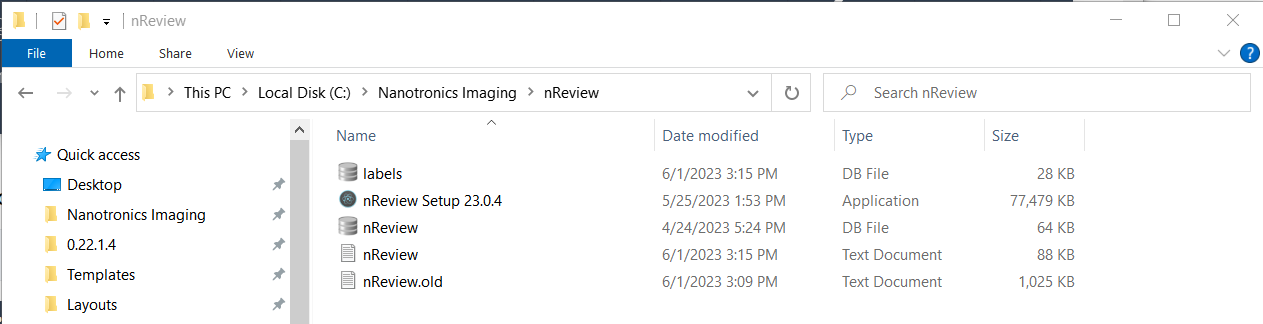
Location of the labels.db file generated by nReview
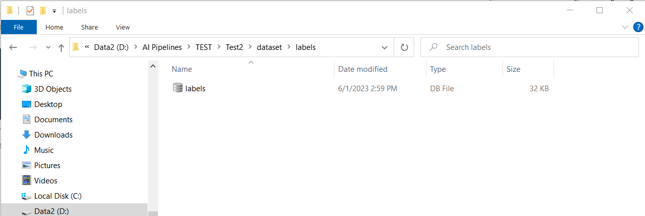
The labels.db file in the nTelligence project folder that should be replaced
Note that in order to add more data to an nTelligence project after completing any amount of work in nTelligence, the labels.db file in the nTelligence project will have to be moved back to the nReview folder, and then additional analyses can be appended to the file via the Label button. Then finally, the labels.db file will need to be moved back into the nTelligence project folder again.
Creating Defect Classes
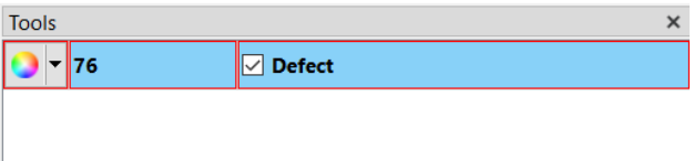
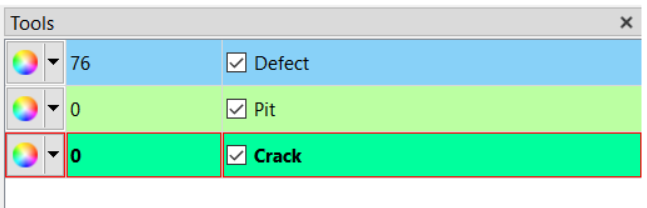
In order to use the Reclassifier Tool, atleast two classes need to be created in the Tools panel in nTelligence.
First, a “defect” class needs to be created. The “defect” keyword is recognized by the Reclassifer Tool as a special class. Importing the nReview labels.db file will automatically label all detected defects with a bounding box and the “defect” class.
Second, atleast one or more defect classes should be added to the class list. These are the defect classes that the Reclassifier will sort the “defect” class defects into. It is highly recommend to add a few unknown classes, e.g. “UNKNOWN1” and “UNKNOWN2”, in case there are defects outside of the known classes that are found in the detection phase.
Using the Reclassifer Tool
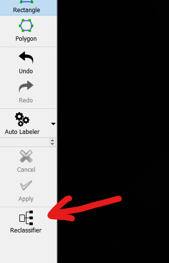
Click the Reclassifer button.
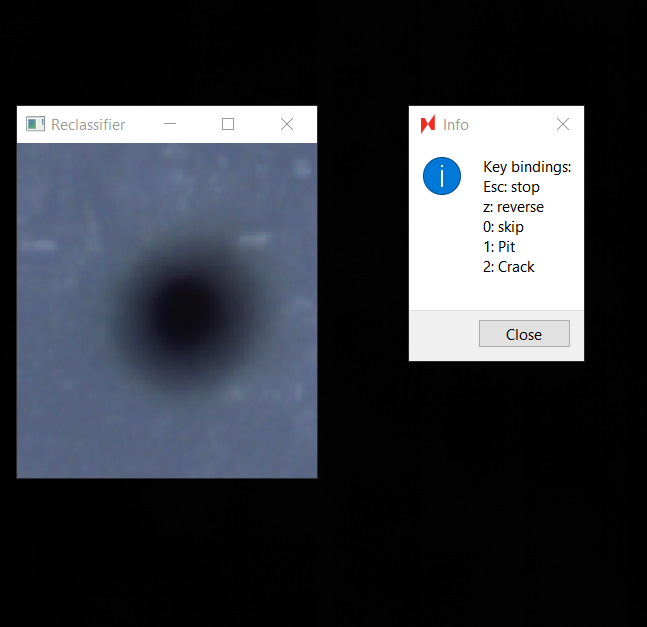
This will bring up two windows. The Reclassifier window shows an image of a defect, and the Info window shows directions for labelling. Now, labelling defects is as easy as pressing the number associated with the defect class of interest.
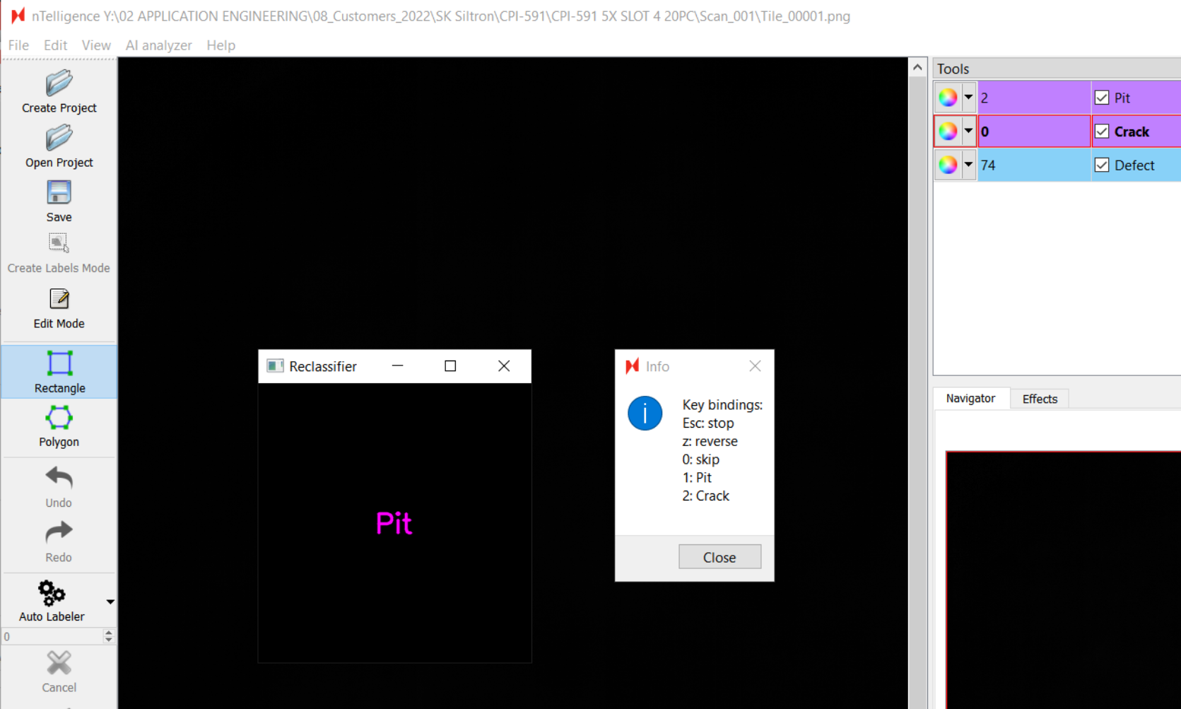
After pressing the appropriate number, in this case 1, the name of the defect will pop up on the Reclassifer window.
Continue to label the defect images until all are labelled. If new defect classes are found during labelling, they can be classified into the “unknown” class labels, with each unique defect class sorted into its own label. The label names can be changed after classification in nTelligence. However, if additional defect classes are not made and new defect types are identified, the user will have to exit the Reclassifer Tool, add the classes, and then start over with classifying all of the defects found. Having “unknown” class labels saves time.
Training the AI
After labelling all defects, begin training a classification model by navigating to AI analyzer > Model.Our recommendation for a classification model is Classifier ResNet18. If that does not give good results, try training on Classifier MobileNetV2 and Classifier Custom, however, preliminary internal testing has shown that Classifier ResNet18 gives best results for most use cases.
After choosing a model, a dialog will pop up asking “Do you want to import a pre-trained model?”. Click No. This allows the model to be trained from scratch.
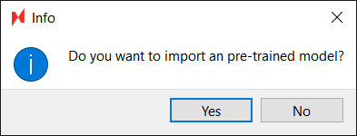
Adjust any parameters – recommend changing the Batch Size to 8 and Num Epochs to 100 – and then click OK to begin training the AI.
Defect Classifier
Overview
To use the Defect Classifier Analyzer, a classification model must be trained with labelled training data.
The classification model file must be trained by Nanotronics applications engineer. To request assistance in training a defect classification model, please contact support@nanotronics.ai to request support.
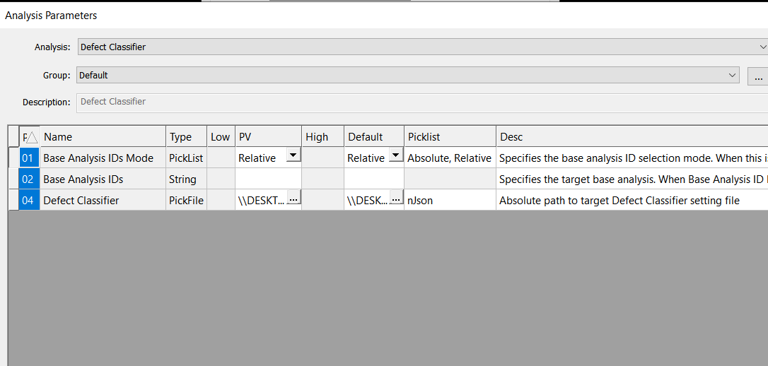
Defect Classifier Analysis
Using the Defect Classifier Analysis
After training an AI to classify defects of interest, the model is ready to be used as part of any nSpec workflow. Defect Classification builds on the results of a base analysis like Basic Selection or Device Inspection. The base analysis is referenced through the Base Analysis IDs parameters.

Surface Prediction Algorithms
Overview
nSpec can automatically predict the surface of any given sample using predictive focus algorithms.
Predictive focus algorithms use the results of the autofocus phase of scanning to estimate the focal plane of the given sample. There are a number of different predictive focus algorithms that can be used to predict and model a sample’s surface topology.
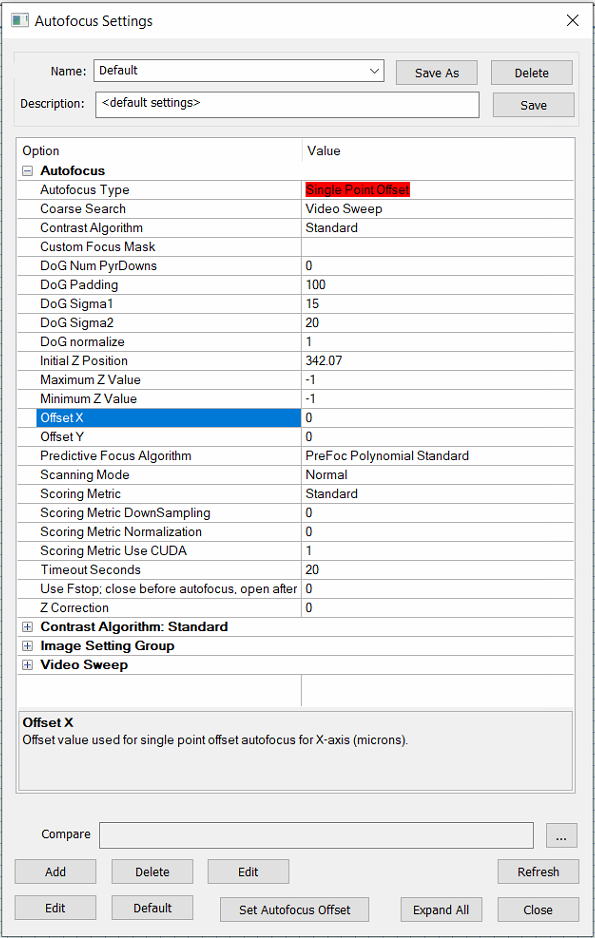
Predictive focus algorithms can be configured and set in the Autofocus Settings dialog, located in Imaging Settings. Users must select Automatic Predictive for Autofocus Type in order to choose a Predictive Focus Algorithm.
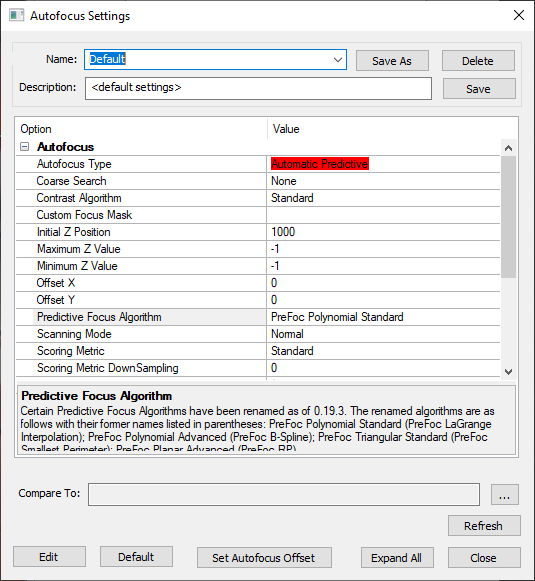
Note that when selecting either the PreFoc Kriging, PreFoc Polynomial Advanced, or PreFoc Planar Advanced algorithms, after selecting the algorithm, users must save the settings in order to see the additional parameter settings appear in the settings dialog.
Autofocus Background
The following diagram gives an overview of how the autofocus phase of scanning works, along with its inputs and outputs. This article will go into detail about the various surface predictor algorithms that can be used as inputs to the autofocus step.
Surface Prediction Algorithms
The six available algorithms are as follows:
PreFoc Polynomial Standard
PreFoc Polynomial Advanced
PreFoc 3CP
PreFoc Triangular Standard
PreFoc Planar Advanced
PreFoc Kriging
In general, using the PreFoc Polynomial Standard option is recommended. If the surface prediction result using this algorithm is not adequate, e.g. does not suffieciently capture or model the sample surface, we recommend using the PreFoc Kriging option instead.
See the table below for more information on what each algorithm is ideal for. Some focus point patterns are incompatible with certain surface prediction algorithms.
Surface Prediction Algorithm | Use Cases | Algorithm Description |
|---|---|---|
PreFoc Polynomial Standard | For general use cases, we recommend this option, which has a fast runtime. Should only be used with a rectangular grid of focus points, which makes it ideal for device scans. | Creates a model of the surface that goes through all focus points, using a polynomial algorithm. Creates a continuous, curved surface. |
PreFoc Polynomial Advanced | Flexible option with many configurable parameters, can be used with irregular focus point pattern, and will cover the edges of a circular wafer especially at higher magnification. More details on the PreFoc Polynomial Advanced algorithm parameters below. | Creates a model of the surface using a polynomial algorithm. Creates a continuous, curved surface. |
PreFoc 3CP | Can be used for irregular, non-square patterns. | Creates a model of the surface using the 3 closest focus points to calculate the Z value of a given point. Creates a non-continuous surface |
PreFoc Triangular Standard | Ideal for low magnification and smooth surfaces. Very fast, easy to configure. Can be used with an irregular focus point pattern. | Creates a multi-plane, non-continuous model of the surface using the 3 focus points that comprise the smallest perimeter triangle around a given point. |
PreFoc Planar Advanced | Can be used with irregular focus point pattern, but should only be used if the sample is known to be a plane. | Creates a single plane model of the surface by calculating a best fit plane through the focus points. There are two parameters: Number of fit attempts, and Objective Depth of Field, which will throw out outlier focus points when calculating the best fit according to a given tolerance. |
PreFoc Kriging | Good for irregular surfaces with nonsquare patterns of many (16+) focus points. Prefer over PreFoc Polynomial Advanced because it is generally faster and more accurate, and covers a similar use case. More details on the PreFoc Kriging algorithm parameters below. | Generates an continuous surface from the focus point z-values, using statistical modeling of all points to make an estimation of the Z value at a given point. |
PreFoc Kriging Parameters
Kriging is a procedure that generates a continuous surface from a set of known focus point z-values. It uses statistical modeling to make an estimation of the Z value at a given point, using some or all of the given z-values, where points closer to the point of interest are more heavily weighted than those further away.
Recommended Settings
We recommend starting with the follow settings and modifying as necessary.
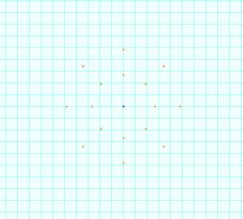
Use Constant for Model Type parameter
Use a 16 point circular predictive focus pattern with 2 rings and 1 center point
Outer ring of 10 points should be near edge of the wafer
Middle ring of 5 points should be halfway between the center point and outer ring
No phase between rings
PreFoc Kriging Parameter Descriptions
Parameter Name | Parameter Values | Description |
|---|---|---|
Krige Type | Simple, Ordinary | Simple is recommended, relates to an assumption about the mean of the focus points. |
Model Type | Constant, Linear, Spherical, Exponential, Gaussian, Power | Type of equation to fit through the focus points. Will relate how the neighboring points influence the estimated z-value at a given point. |
Neighboring Points | Number, 1 up to number of focus points. | The number of neighboring points to use when estimating the z-value for a given point. |
Range | Number, up to the diameter of the sample. | Specifies the distance from a point of interest to consider as influential to that point of interest. Points outside of this boundary will influence the estimated z-value much less. Usually a large value. |
Sill | Number | This number is the variance in z-values for points outside of the range. Should not be used with the Power model type, instead set when using the Exponential model type parameter. |
Exponent | Number | If using the Power model type, this parameter sets the degree of the exponent. |
PreFoc Polynomial Advanced Parameters
PreFoc Kriging is preferred over PreFoc Polynomial Advanced for the same use case, as it is more accurate. However, if you’d like to experiment using the PreFoc Polynomial Advanced surface prediction algorithm, feel free to tweak the following parameters.
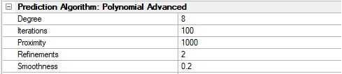
PreFoc Polynomial Advanced Parameters Description
Parameter Name | Parameter Range | Description |
|---|---|---|
Degree | 2 to 15 | This is the polynomial degree, e.g. 2 is quadratic, 3 is cubic, etc. This is the parameter that controls the behavior of the whole algorithm and should be adjusted first. The degree is the number of undulations in one linear direction across the wafer. For example, a bowl shaped wafer, which is pretty common due to suction, will need degree 2: down and then up undulation. Odd degrees will create non-symmetric undulations and should be avoided but may work in some cases. |
Refinements | 0 to 3 | The number of times the algorithm subdivides the surface in between the focus points for greater detail. Choosing 1 will divide the surface in half, 2 will divide in quarters, and so on. The greater the number of refinements, the slower the algorithm. This can be experimented with for fine adjustment, 1-3 is ideal. |
Iterations | 0 to 1000 | After refinement, the final surface is fit. This is the number of iterations the algorithm will perform to adjust the fitted surface numerically. This parameter value can go up to a 1000 in steps of 100. This can be experimented with for fine adjustment. |
Proximity | 0 to 1000 | This parameter determines how close the surface passes through the focus points. 1000 means the surface passes exactly through the focus points, and 10 or 100 means approximately. This is a weight so is independent of distance. |
Smoothness | 0 to 1 | This is a constraint on how smooth the final surface should be during fitting. It is a scalar value between 0 and 1, where 1 is a very smooth/flat plane. This value can be decreased with the use of a lot of focus points, but if very few focus points are used with a high degree, smoothness can be increased to guarantee a more natural surface. |
Flat Plane Surface Predictor
Overview
It is recommended that all scans use a surface predictor, unless running autofocus on every tile during scanning. Autofocus surface prediction types Manual Set and None/Manual have been replaced by a new Flat Plane surface predictor which creates a flat plane from a given Z value, or the current stage Z value.
Flat Plane Surface Predictor Replaces Manual Set, Manual, and None Autofocus Types
Imaging Settings Dialog Updates
Overview
There are a number of exciting updates in nSpec v0.23.0.0 to filter and lighting functionality and UI.
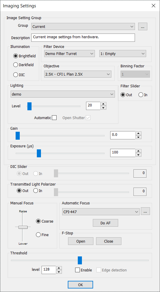
Imaging Settings Dialog
Lighting
The previous UI supported only two light sources, an A and B light source. Now, nSpec supports any number of different light sources, accessed via the Lighting dropdown. Multiple light sources can be set at a time, with each source being set individually in the Image Settings Group, as seen below.
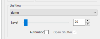
Lighting section of Imaging Settings Dialog
These changes in also reflected in the Current Image Settings section of Scan Settings.
Filter Devices
The Filter Device dropdown allows the user set the active slot used for a number of different filter devices. The dropdown to the right is populated with each filter device’s available slots or modes. Typically, most nSpec machines will only contain one filter device. This device could be a Nanotronics filter cube used with fluorescent illumination modes, a Nanotronics filter wheel used to filter white light for machines with Olympus illuminators, and filter sliders used for filtering white light from other illumination sources, like the Thorlabs filter slider.
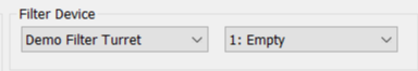
Filter Device Section of Imaging Settings Dialog
In v0.23.0.0, the neutral density filter is controlled in a separate area of the Image Setting Group, and is used to reduce light intensity.
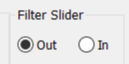
Filter Slider Section of Imaging Settings Dialog
Device Layout Editor Updates
Overview
The nSpec Device Layout Editor has been redesigned for clarity and usability. Additionally, it also includes some new features as well, for example, the ability to create a device layout that fills an entire circular wafer, given the diameter and edge exclusion values.
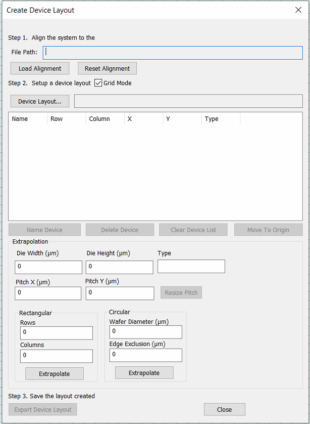
Creating a Device Layout using Circular Extrapolation
First, specify an alignment file and input the die and pitch measurements in the extrapolation section. Next, input the wafer diameter and edge exclusion values and click Extrapolate. This will allow users to extrapolate radially from the origin point, which is defined by the alignment file.
After clicking Extrapolate, we recommend viewing the sample layout via the stage view, and adjusting the die and pitch values to as necessary to achieve an accurate device layout file. Click Export Device Layout to export and save the generated device layout.
Sample Naming and Wafer Skipping Behavior
For nSpec PS systems that are running jobs on cassettes, users have the ability to exclude specific wafers in a cassette from being scanned.
There are two main ways to implement this functionality: first, through the Sample ID List utility, and second, through manual input in the Scan Setting dialog's Sample field. Note that in these notes, wafer and sample are used interchangeably, but the Sample field in the Scan Setting dialog has a more ambiguous meaning, which is detailed in the following sections.
Breaking Change to Skip Behavior
Prior to nSpec v0.23.0.0, the use of a semicolon in the Sample name or Sample ID fields denoted wafer-skipping behavior.
Starting with nSpec v0.23.0.0, only _SKIP_ will denote wafer-skipping behavior, and using a semicolon will no longer indicate skipping.
Navigating the Sample ID List Utility
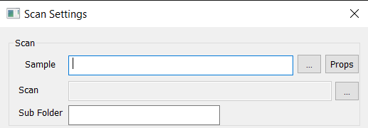
The skip wafer functionality is embedded into the Sample ID List utility, which is found at Stage View > Scan > Sample > "...". This utility helps construct a Sample name that has the wafer skipping behavior encoded, and also allows users to give individual wafers in a cassette, unique sample names.
Clicking “…” opens the Sample ID List dialog
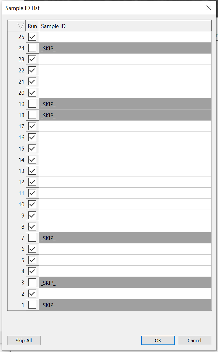
Sample ID List dialog
In the above Sample ID List dialog, checking the checkbox for a given wafer will include it in the scan, and unchecking it will skip it and automatically input _SKIP_ as that wafer’s Sample ID. The bottom left "Skip All" button seen in the above Sample ID List dialog will deselect all checkboxes when toggled. When all checkboxes are unchecked, the button changes to "Scan All", allowing the user to select all the checkboxes.
The above Sample ID List dialog would generate ;_SKIP_;;;;_SKIP__SKIP_;;;;;;;;;;_SKIP_;;;_SKIP_;_SKIPin the Scan > Sample field entry, with each scanned wafer encoded as a single semicolon and each skipped wafer encoded as _SKIP_.
In the above screenshot, the Sample ID List utility helps encode a Sample name in the Scan Settings dialog of SiC;_SKIP_;C. This means the first and third wafers will be scanned, and include and C and SiC in their Sample ID names, and the second wafer will be skipped entirely.
Sample Naming Behavior
Users can also forego using the Sample ID List dialog, and directly input the Sample name in the Scan Settings dialog found atScan Settings > Scan > Sample.
There is different sample naming and skipping behavior depending on if the user is using an autoloader with an OCR to obtain sample IDs or not. These behaviors are detailed in the following table.
Sample Behavior When Using an Autoloader
In the following table, the wafer ID obtained via the autoloader OCR is denoted as OCR_ID.
Input in | Scan using OCR | Scan without OCR or with job property |
|---|---|---|
Blank or empty set of semicolons ( | Every sample will be uniquely named using its own | Invalid, job will fail |
| Every sample will be uniquely named using | Every sample will be named as |
| Invalid, job will fail | Invalid, job will fail |
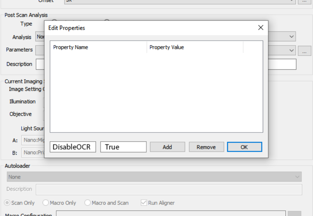
When job property DisableOCR is enabled on a multi-job, it is set for the whole recipe. It cannot be set differently per job in a multi-job.
The job propretyDisableOCR can be enabled or disabled using the Edit Properties dialog found at Scan Settings > Job > Props. The sample naming and skip behavior listed in the above table is the same whether running a single or multi-job with autoloader.
Sample Behavior When Manually Loading Sample
When manually loading samples in a single or multi-job without the autoloader, the user must input some arbitrary_textinto the Scan Settings > Scan > Sample field to be used as the name for each sample, otherwise the job will fail as there is no OCR present to obtain each wafer’s ID to use for its sample name.
New Features
Overview
There are a huge number of new features and workflows included in nSpec v0.23.0.0. Smaller features are documented below, while major features and workflows have separate documentation.
Highlights
NSPEC-4041: Ability to add XY offset parameters to Autofocus
Users can now add offsets to their autofocus routines via Offset X and Offset Y fields (units are in µm) in the Autofocus settings dialog. Note that the offset parameters are enabled only when the Autofocus Type is set to Single Point Offset. Additionally, the autofocus routine must be for a Device Inspection scan. During the autofocus routine, autofocus is performed for each device at the offset location. If the Autofocus Type is set to Single Point Offset and the autofocus settings are applied to a non-Device Inspection scan, autofocus will simply not run at all.
NSPEC-4244: New job properties allow users to filter devices to be scanned
New job properties ScanSingleDeviceIndex, ScanStartDeviceIndex,ScanSingleDeviceIndex allow users to filter and specify which devices should be scanned.
ScanSingleDeviceIndex given a device ID, will only scan the specified device.
ScanStartDeviceIndex given a device ID, starts the scan at the given device ID.
ScanUpToDeviceIndex given a device ID, will scan up until the given device ID.
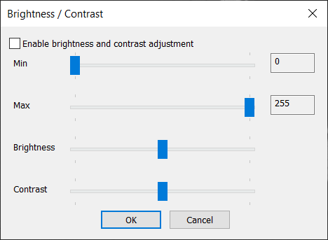
NSPEC-4510: Ability to change brightness/contrast of nSpec Live View
This dialog is reachable via nScan - Camera View> View > Adjust brightness contrast...
No update to the live view image will be shown though until the Enable brightness and contrast adjustment checkbox is enabled. Closing the dialog will disable this view, as will deselecting the checkbox.
NSPEC-5594: New Custom Exporter Outputs (KLARF, JSON, XML)
The Custom Exporter launched in nSpec version v0.22.1.0 with support for CSV exports. With this change the Custom Exporter now supports KLARF, JSON, and XML exports as well. For full documentation on this feature please see the Custom Exporter Appendix page, or at Custom Exporter
NSPEC-5916: Tilt removed from Flatness Report PNG
When viewing the exported Flatness Report PNG file, the report will now display data that has been corrected for any tilt present in the stage, as determined by Predictive Autofocus.
However, when viewing the Flatness Report within nView, the rendering will continue to show the original raw data, which includes tilt. This enables users to perform troubleshooting tasks using the Flatness Report in nView, for example, visualizing any tilt present.
The accompanying exported focus point CSV file will continue to contain the original raw focus point data.
See Appendices section for more on flatness reports.
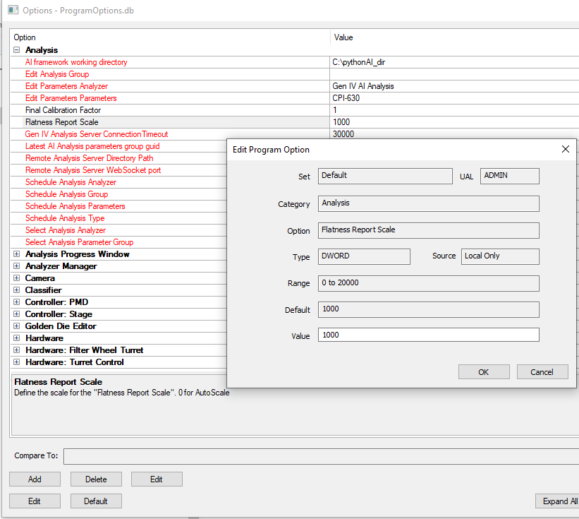
NSPEC-6683: New Flatness Report Scale program option allows user to set custom manual scale when viewing flatness report
In addition to the existing autoscale mode, the flatness report scale can now be set to a fixed scale in the Program Options dialog, with the parameter value as the scale maximum in microns.
NSPEC-6908: Add the Cropped Image Analysis data into the database
After running the Cropped Image Analysis, the resulting data will be added to the database. This allows for the cropped image defect data to be used with tools like Custom Reporter and Custom Exporter.
NSPEC:6970: Improved Keyboard Control of nSpec Axes
There are improved keyboard controls for controlling the nSpec Axes. Holding Shift down while using the arrow keys will move the X/Y axes quickly, with speeds independent of the objective. Holding CTRL down will move the X/Y axes 1-unit step at a time for slow and precise movement. Using arrow keys on their own will move at speeds dependent on the Field of View for X/Y axis movement, and dependent on the Depth of Field for Z axis movement.
NSPEC-7180: Program Option for Disabling Door Unlock at the End of a Job
New program option Automate Interlock Unlocking under the Scanning category, can be set to either 0 or 1. If 0, the interlock(s) only unlock when the user explicitly chooses to unlock by toggling nScan - Stage View > Door > Lock Door, and if 1, nSpec will automatically unlock the interlock(s) after job completion and after specific actions. This option defaults to 0.
NSPEC-7256: New Stage Initialization Z-Height
Previously, when starting up nSpec, the stage would initialize at whatever the last known Z-height was. Now, the stage initializes to the middle of the Z-range. If a custom start position is desired, it can be set at the program option under the Controller: Stage section by setting the Initial X Position, Initial Y Position, and Initial Z Position parameters.
New Features Changelog
Bug Fixes
Highlights
NSPEC-6267: Interlocks don’t re-engage Stage
When the interlock on an enclosure unlocks, power is killed to the stage for safety reasons. However, when the door is shut and the interlock is locked again, the stage is not re-engaged until after the first motion. This causes a few problems:
The first scan after the interlock was touched was captured at the incorrect position
If the first motion is for an alignment job, first alignment mark will be missed
These problems have now been fixed! After open an interlock-equipped system door and closing it, stage motion will be immediately reset.
Make sure to set the program option in the PMD category called Use Interlock Recovery to 1
NSPEC-6363: F-stop opens and closes for every autofocus point
Previously, there was unexpected behavior where the F-stop opened and closed for every autofocus point. Now, the F-stop stays closed for the duration of the autofocus procedure, as expected. This fix should increase the longevity of the F-stop belt and motor.
NSPEC-6469: If first job in a job group for multiple wafers is set with job properties, first job ignored
This release includes a bug fix in which the first job in a job group will be ignored if A) the autoloader is used, B) the job group is being performed on multiple wafers, C) the first job is set with job properties.
For example, if running a job group on multiple wafers and the first job is set with the job property to export a flatness report, the flatness report will not be exported but all other subsequent jobs will be performed.
NSPEC-6479: Group job does not work if SampleID empty
Group jobs fail after the first scan if it is an Autoloader job and SampleID is left empty.
NSPEC-6615: Defect data not reported in CSV file from Cropped Image Analyzer
Defect data is now reported in the CSV file following Cropped Image Analysis.
NSPEC-6884: Custom Reporter broken in recent patch releases
Custom Reporter is fixed and runs successfully.
Changelog
Known Issues
NSPEC-7525: Revert to Old Behavior for NSPEC-7460
A patch will be released that will fix alignment search optimization, which is enabled via a program option. Until then, we do not recommend using this program option, and recommend using standard alignment procedures instead.